Chapter 3.5: How might the virus spread in the future?
Without sufficient data, it’s virtually impossible to predict exactly how the virus will spread. There are too many unknown variables: how county policies will change, how compliant citizens will be, if and how the virus may evolve, and whether or not health care systems will be able to accomodate new cases.
There are tools that can extrapolate possible predictions, but the results are based on the assumption that nothing changes, which is highly unlikely. Understanding the bias that this method introduces, I used a package called curvefit to predict the course of the virus in different counties and where the infection count may cap.
import pandas as pd
import requests
import numpy as np
import matplotlib.pyplot as plt
from functions import calculate_infection, detection_plot, clean_deaths, clean_cases
from scipy.optimize import curve_fit
deaths_df = pd.read_csv('https://raw.githubusercontent.com/CSSEGISandData/COVID-19/master/csse_covid_19_data/csse_covid_19_time_series/time_series_covid19_deaths_US.csv')
deaths_df = clean_deaths(deaths_df)

deaths_df_HR = deaths_df.iloc[362,:]
deaths_df_HR = deaths_df_HR.reset_index()

index_val = len(deaths_df_HR.index)

calculate_infection(deaths_df_HR, index_val)
deaths_df_HR = deaths_df_HR[0:-18]

index_val = len(deaths_df_HR.index)
Miami-Dade County
def logistic(x, midpoint=0, rate=.8, maximum=1):
    return maximum / (1 + np.exp(-rate * (x - midpoint)))

x = np.linspace(-6, 10, 1000)
y = logistic(x)# + logistic(x, midpoint=6, rate=2, maximum=5)


def double_log(x, x1, r1, m1, x2, r2, m2):
    return logistic(x, x1, r1, m1) + logistic(x, x2, r2, m2)


popt1, _ = curve_fit(logistic, range(0, index_val),  deaths_df_HR['total_infections'], p0=[0,0,0])

popt2, _ = curve_fit(double_log, range(0, index_val), deaths_df_HR['total_infections'], p0=[0,0,0,0,0,0])

xmodel = np.linspace(-10, index_val, 1000)
ymodel1 = logistic(xmodel, *popt1)

ymodel2 = double_log(xmodel, *popt2)

plt.figure(figsize=(12,8))

plt.plot(xmodel, ymodel2, 'r')

yy = deaths_df_HR['total_infections']
xx = range(len(deaths_df_HR['total_infections']))
plt.scatter(xx,yy)

print(popt2[2] + popt2[-1])
497236.99904814764
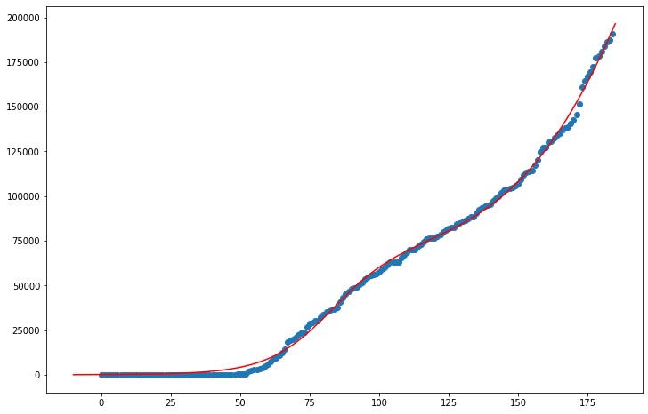
The data points for Miami-Dade don’t appear to be on a flattened trajectory yet, whereas the curvefit model suggests that Miami-Dade will reach its maximum number of infections relatively soon. When exactly Miami-Dade will turn over cannot be determined, especially with estimates as crude as these, but I estimate the maximum number of infections to be around 200,000.
deaths_df_CK = deaths_df.iloc[610,:]
deaths_df_CK = deaths_df_CK.reset_index()

index_val = len(deaths_df_CK.index)

calculate_infection(deaths_df_CK, index_val)
deaths_df_CK = deaths_df_CK[0:-18]
index_val = len(deaths_df_CK.index)
Cook County
def logistic(x, midpoint=0, rate=.8, maximum=1):
    return maximum / (1 + np.exp(-rate * (x - midpoint)))

x = np.linspace(-6, 10, 1000)
y = logistic(x)# + logistic(x, midpoint=6, rate=2, maximum=5)


def double_log(x, x1, r1, m1, x2, r2, m2):
    return logistic(x, x1, r1, m1) + logistic(x, x2, r2, m2)


popt1, _ = curve_fit(logistic, range(0, index_val),  deaths_df_CK['total_infections'], p0=[0,0,0])

popt2, _ = curve_fit(double_log, range(0, index_val), deaths_df_CK['total_infections'], p0=[0,0,0,0,0,0])

xmodel = np.linspace(-10, index_val, 1000)
ymodel1 = logistic(xmodel, *popt1)

ymodel2 = double_log(xmodel, *popt2)

plt.figure(figsize=(12,8))

plt.plot(xmodel,ymodel2, 'r')

yy = deaths_df_CK['total_infections']
xx = range(len(deaths_df_CK['total_infections']))
plt.scatter(xx,yy)


print(popt2[2] + popt2[-1])
489353.2772729657
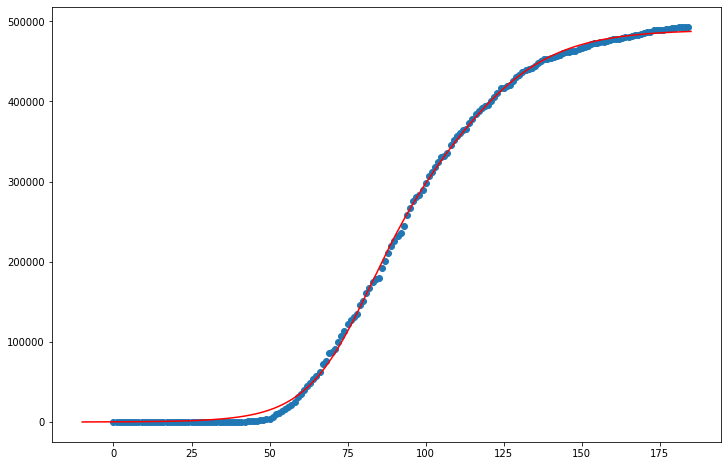
The data for Cook county thus far suggests that COVID 19 infections have nearly turned over, and the virus may have run its course. The curvefit model doesn’t appear to have much work to do, with such a normalized and complete infection estimate thus far. Unless Cook has another spike in infections, this model is probably fairly accurate in assuming that the maximum number of infections is nearly half a million.
deaths_df_LA = deaths_df.iloc[204,:]
deaths_df_LA = deaths_df_LA.reset_index()

index_val = len(deaths_df_LA.index)

calculate_infection(deaths_df_LA, index_val)
deaths_df_LA = deaths_df_LA[0:-18]

index_val = len(deaths_df_LA.index)
Los Angeles County
def logistic(x, midpoint=0, rate=.8, maximum=1):
    return maximum / (1 + np.exp(-rate * (x - midpoint)))

x = np.linspace(-6, 10, 1000)
y = logistic(x)# + logistic(x, midpoint=6, rate=2, maximum=5)


def double_log(x, x1, r1, m1, x2, r2, m2):
    return logistic(x, x1, r1, m1) + logistic(x, x2, r2, m2)


popt1, _ = curve_fit(logistic, range(0, index_val),  deaths_df_LA['total_infections'], p0=[0,0,0])

popt2, _ = curve_fit(double_log, range(0, index_val), deaths_df_LA['total_infections'], p0=[0,0,0,0,0,0], maxfev = 20000)

xmodel = np.linspace(-10, index_val, 1000)
ymodel1 = logistic(xmodel, *popt1)

ymodel2 = double_log(xmodel, *popt2)

plt.figure(figsize=(12,8))

plt.plot(xmodel, ymodel2, 'r')

yy = deaths_df_LA['total_infections']
xx = range(len(deaths_df_LA['total_infections']))
plt.scatter(xx,yy)

print(popt2[2] + popt2[-1])
603161.6180678995
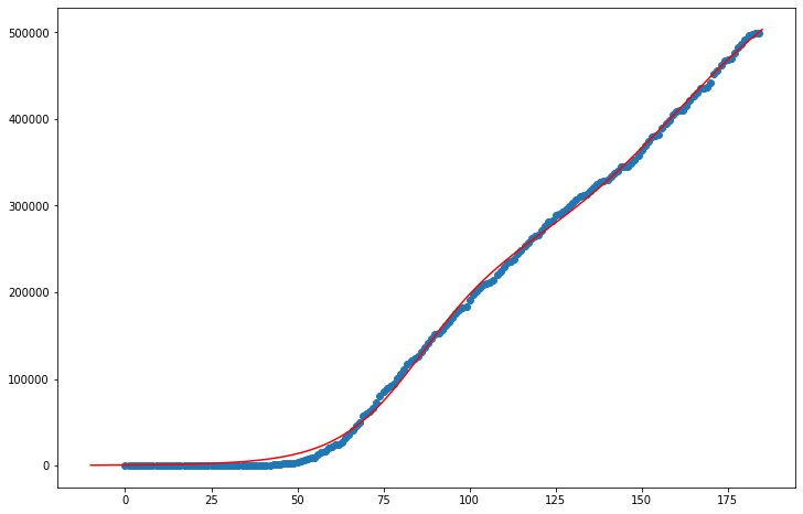
The data points for Los Angeles appear to continue to rise at a linear rate, if not exponential. This model, however, indicates infection numbers will turn over soon, and thus the maximum potential number of infections isn’t much greater than the current number of estimated infections. With a population of over 10 million people, I would say that LA’s potential number of infections is much higher than the model’s estimate of 450,000.